In a recent project, I have developed a gradient boosting algorithm to estimate price elasticities. Surely, it is necessary to validate if the functionalities of the algorithm are working as intended. I started using nonlinear time series data from another blog post about lag selection as a validation basis. Unfortunately, at that time I did not wrap the simulation code into a time series simulation function. Thus, I wondered whether there are any simulation packages or functions for supervised learning problems. My colleagues were confronted with a similar problem and they have used the simulation functions developed by Max Kuhn in his supervised learning framework ⁽¹⁾. I started using LPH07_01() to validate whether features of the underlying data generating process were really selected. While the function does its job as expected, I realized that I needed more degrees of freedom in my simulation. One of the crucial settings I wanted to manipulate is the degree of nonlinearity and the associated functional shape, since the boosting algorithm uses P-spline⁽²⁾ base learners. At this point, I decided to code my own simulation function and yep here it is. The function is called Xy() and you can get it from my github account.

Main functionalities of my simulation are salvaged from the counterpart. For instance, one can add irrelevant features and multicollinearity within . However, Xy() is additionally allowing collinearity patterns between relevant and irrelevant features. Nonlinearity is completely adjustable by manipulating the nlfun argument. Additionally, an interaction depth can be specified via the interaction parameter. Altering this argument does however not imply that will be completely generated by interactions. Chance will decide for each true feature whether an interaction should be formed. For instance, if the user decides in favor of an interaction depth of – say – two, it is likely that will be generated by some bivariate interaction terms.

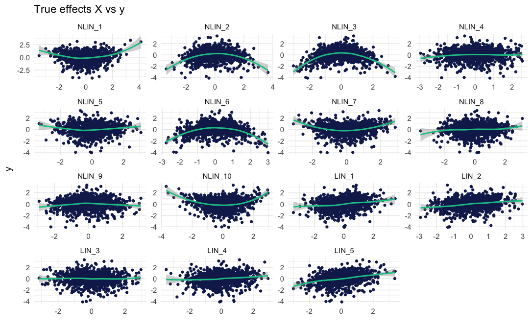
In this example, we can see that the process generating is composed of main and interaction effects of degree two.

# Simulating regression data with 15 true and 5 irrelevant features
reg_sim = Xy(n = 1000,   
             linvars = 5,    
             nlinvars = 10,   
             noisevars = 5,   
             nlfun = function(x) {x^2},  
             interaction = 2,  
             sig = c(1,4),   
             cor = c(0.1,0.3),  
             weights = c(-5,5),  
             cov.mat = NULL,  
             sig.e = 4,  
             noise.coll = FALSE, 
             plot = TRUE)  

# Get the underlying process of y 
reg_sim[["dgp"]]  

"y =  3.74NLIN_1 - 4.48NLIN_2 * -3.54NLIN_3 - 2.39NLIN_3 * -2.27LIN_4
    - 1.45NLIN_4 + 2.67NLIN_5 * -4.17LIN_3  
    - 3.63NLIN_6 - 2.39NLIN_3 * 4.66NLIN_7 + 0.77NLIN_8  
    - 0.42NLIN_9 * 1.93LIN_2 - 2.27NLIN_9 * 0.29NLIN_10 - 1.49LIN_1  
    + 1.39LIN_2 + 4.43NLIN_10 * 3.6LIN_3 - 3.26NLIN_6 * 3.51LIN_4  
    + 4.47LIN_1 * 4.38LIN_5 + e ~ N(0,4)"

I liked the idea of a user-specified interval from which variances of the true features are sampled, since this opens the possibility to play around with different variations. The covariance of as well as the weights of are also sampled from a user specified interval. If you have a specific covariance structure in mind you can define it by using the cov.mat argument.

The function returns a list with the simulated data, a string describing the composition of and if applicable a plot of the true effects.

Here are the true effects of our example:

The function comes with a ⁽³⁾ body which should – hopefully – clarify the tasks of each argument.

There are several things I want to add in upcoming versions. On top of my list are classification tasks, binary or categorical features in general, data with autocorrelative patterns and a user-specified formula describing the composition of .

I hope you enjoy this simulation tool as much as I do. As mentioned above, I did not actively search CRAN for simulation packages or functions, so if you know a good package or function you can drop me an e-mail. Also, feel free to contact me with input, ideas or some fun puppy pictures.

Referenzen

1. Kuhn, Max. „Caret package.“ Journal of statistical software 28.5 (2008): 1-26.
2. Eilers, Paul HC, and Brian D. Marx. „Flexible smoothing with B-splines and penalties.“ Statistical science (1996): 89-102.
3. Wickham, Hadley, Peter Danenberg, and Manuel Eugster. „roxygen2: In-source documentation for R.“ R package version 3.0 (2013).

Über den Autor

André Bleier

The most exciting part of being a data scientist at STATWORX is to find this unique solution to a problem by fusing machine learning, statistics, and business knowledge.