Macbeth shall never vanquish'd be until

Great Birnam Wood to high Dunsinane Hill

Shall come against him. (Act 4, Scene 1)

In Shakespeare's The Tragedy of Macbeth, the prophecy of Birnam Wood is one of three misleading prophecies foreshadowing the defeat of the protagonist of the same name. While highly unlikely, the event of a nearby forest moving towards his castle marks the beginning of Macbeth's doom.

This blog post likewise centers on a (greedy) forest having the potential to overthrow a ruling king. It is about a direct decision forest learning algorithm threatening the dominance of Gradient Boosting Decision Trees (GBDT) for problems in machine learning requiring to learn nonlinear functions from training data.

Recap Gradient Boosting Decision Trees

Before turning to the prophecy, let us explore one of the most widely applied machine learning techniques – Gradient Boosting Decision Trees. Given a nonlinear function with input , we want to find a suitable prediction function with training data by minimising an arbitrary loss function:

   

Gradient Boosting solves this problem by fitting an additive model:

   

with base learners characterised by and step size . For the case of a quasi least-squares regression (), the complete algorithm, can be summarised as follows (Friedman 2001):

1. Set the initial model , where is the empirical mean of all training data.

2. For each boosting iteration :

   1. Compute the residual vector , which is equivalent to the negative gradient .
   2. Fit a base learner to the negative gradient vector and obtain by:
   3. Find the optimal step size by
   4. Update model:

In order to control overfitting, the line 2.4 is normally replaced by , where is the shrinkage parameter (or learning rate).

Motivation

While GBDT is among the most successfully applied machine learning algorithms, its design is not above all doubt. Johnson et al. (2014) point out three shortcomings of the general boosting framework outlined above:

1. A lack of explizit regularization
2. Huge models in terms of boosting iterations due to small step sizes
3. Base learner treated exclusively as black boxes

The first criticism is especially interesting. While modern implementations of boosting, like XGBoost and LightGBM, add explicit regularization terms, the general boosting framework does not. It is often argued, that the combination of small step sizes and frequent boosting iterations act as an implicit regularization (Hastie et al. 2009). While this is certainly true, it is still unclear in which way those implicit regularization techniques interact with each other and whether this interaction is optimal or not (Rosset et al. 2004, Johnson et al. 2014).

As a result of this regularization technique, the small step sizes, lead to more complex models that need long boosting paths. Besides the small step sizes, performing only a partial corrective step in every iteration is another reason that calls for long boosting paths. More precise, in GBDT the parameter vector gets optimized only for the current model while all previous models remain untouched (see 2.4). This is what we call forward stagewise additive modeling. Warmuth et al. (2006) argued that a fully-corrective step, where all parameters get optimized in every iteration , can significantly accelerate the convergence of boosting procedures, hence making small step sizes redundant.

A Regularized Greedy Forest

The Regularized Greedy Forest (RGF) extends the general boosting framework by the following three ideas:

1. Add an explicit regularization function
2. Perform fully-corrective steps
3. Add structured sparsity based on the forest structure

The Idea of a Decision Forest

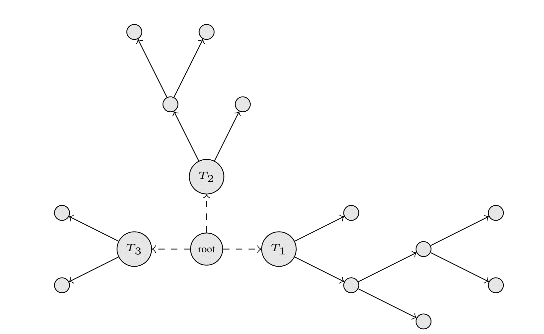
As in GBDT, RGF uses a forest composted of multiple decision trees . Each consists of nodes and edges . Each is associated with a splitting variable and a corresponding splitting threshold . For a better understanding of the later fully-corrective steps, it helps to visualise in it's entire structure (see figure below).

If is a forest with nodes , it can be written as an additive model over all nodes:

   

where is a nonlinear decision rule (basis function) at node . Hence, can be summarized as the product of single decisions of the form along the path from the root to ; is a weight assigned to (for more details on the weight see Hastie et al. 2009, p. 312). Furthermore, the regularized loss function can be expressed as:

   

Implementation of Greedy Optimization

In order to minimize , one can either change the forest structure by changing the basis functions or change the weights . The GBDT algorithm does both in an iterative alternating way.

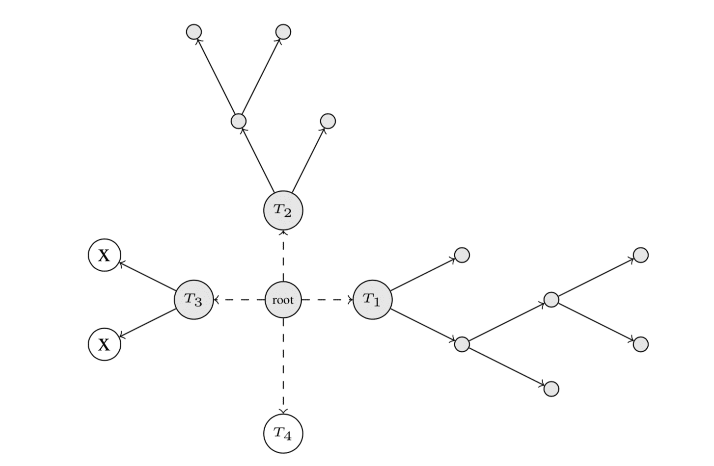
For the structural change, two options are allowed: (1) split an existing leaf, or (2) start a new tree. Both options are displayed in the figure below, where is split in two new nodes and is a new tree starting from the root.

On the computation side, one step of structure-changing operation from the current forest to the new forest can be done by considering the loss reduction resulting from splitting a node with parameters into and . Hence, find . Johnson et al. (2014) suggested to use Newton's method based on the first and second order partial derivatives of to solve the optimisation problem. This is a slightly different approach compared to GBDT where gradient-descent approximation is normally used. Having fixed a new structure of the forest, the second step involves optimising the weights while keeping the structure fixed.

Tree-structured Regularization

Recall that the partial corrective step in combination with small step sizes acts as an implizit regularization for the GBDT. Since the RGF does a fully-corrective step, which does not involve a step size, it needs a more explizit regularization to prevent overfitting.

Johnson et al. (2014) suggested to use a tree-structured penalization technique derived from the grouped lasso (Yuan and Lin 2006). In the grouped lasso, sparsity is enforced by applying the norm penalty on prior known groups of features instead of individual features. Hence, a group of features shares a common penalty. Zhao et al. (2008) generalized this regularization theme by suggesting to assume the feature to form a tree structure (see als tree-guided group lasso in Kim and Xing (2010)). Johnson et al. (2014) leverage this idea by using the already available forest structure as a grouping schema. More precise, they define a shared regularization penalty for all trees sharing a similar topology. Thus, if two trees have an equivalent (see the original paper for a detailed explanation of equivalence) structure, their weight vectors share a common penalty term.

Without going to must into details, Johnson et al. (2014) suggested three different tree-structured regularizers including a simple norm regularizer on the leaf weights :

   

Summary

Regularized Greedy Forest (RGF) is another tree-based sequential boosting algorithm. It differs from the more common gradient boosting framework in three aspects. First, RGF applies fully-corrective steps, which means updating all parameters and weights for all trees (the forest) in every iteration. Second, RFG optimizes an explicitly regularized loss function. Third, RGF leverages the forest structure by imposing a tree-structured regularization technique.

This blog post summarized the most important theoretical aspects of RGF. In the next post, we will apply RGF to various real world problems and compare its speed and performance with GBDT to see whether RGF is the new go-to algorithm in applied data science. Until then, keep Macbeth's words in good memory:

That will never be.

Who can impress the forest, bid the tree

Unfix his earthbound root? (Act 4, Scene 1)

Appendix – RGF in Competitions

• 1st place in Bond Price Prediction (www.kaggle.com/c/benchmark-bond-trade-price-challenge)
• 4th place in Biological Response Prediction (www.kaggle.com/c/bioresponse)
• 1st place in Predicting days in a hospital – $3M Grand Prize (www.heritagehealthprize.com/c/hhp)

References

• Johnson, Rie and Tong Zhang. 2014. "Learning Nonlinear Functions Using Regularized Greedy Forest." IEEE Transactions on Pattern Analysis and Machine Intelligence, Vol. 36, No. 5.
• Warmuth, Manfred K., Jun Liao, and Gunnar Rätsch. 2006. "Totally Corrective Boosting Algorithmus that Maximize the Margin." Proceedings of the 23rd International Conference on Machine Learning, Pittsburgh, PA.
• Hastie, Trevor, Robert Tibshirani, and Jerome Friedman. 2009. "The Elements of Statistical Learning." 2nd Edition. Springer, New York.
• Yuan, Ming and Yi Lin. 2006. "Model selection and estimation in regression with grouped variables." Royal Statistical Society, Vol. 68, No. 1.
• Zhao, P., Rocha, G., and Yu, B. 2008. "Grouped and hierarchical model selection through composite absolute penalties." Technical Report 703, Department of Statistics, University of California, Berkeley.
• Kim, Seyoung and Eric P. Xing. 2010. "Tree-Guided Group Lasso for Multi-Task Regression with Structured Sparsity." Proceedings of the 27th International Conference on Machine Learning, Haifa, Israel.
• Rosset, Saharon, Ji Zhu, and Trevor Hastie. 2004. "Boosting as a Regularized Path to a Maximum Margin Classifier." Journal of Machine Learning Research, Vol. 5, No. 1.